モチベーション
散布図から関数を予測したい
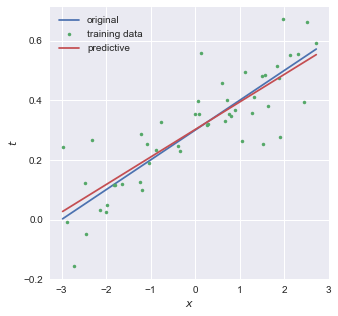
scikit-learnのLinearRegressionで単回帰する
-3 < x < 3 の範囲でxをランダムに50点生成し,
scikit-learnのLinearRegressionを用いて
coefficientは0.09くらい,interceptは0.30くらいとなり,
import numpy as np
from matplotlib import pyplot as plt
from sklearn.linear_model import LinearRegression
from sklearn.model_selection import train_test_split
from matplotlib.colors import ListedColormap

colors = ['#e74c3c', '#3498db', '#1abc9c', '#9b59b6', '#f1c40f'] # red, blue, green, purple, yellow
cmap = ListedColormap(colors)
plt.style.use('seaborn')

def f(x):
    return  0.1*x + 0.3

N = 50
X = np.zeros((N,1))
np.random.seed(seed=10)
X[:,0] = np.random.uniform(-3, 3, N)
noise = 0.1*np.random.randn(N) # σ=0.1
t = f(X[:,0])+ noise

X_train, X_test, t_train, t_test = train_test_split(X, t, random_state=0)

lr = LinearRegression().fit(X_train, t_train)
print("train R^2:", lr.score(X_train, t_train))
print("test R^2:", lr.score(X_test, t_test))
print(f"coefficient:{lr.coef_} intercept:{lr.intercept_}")

fig = plt.figure(figsize=(5,5))


Xcont = np.linspace(np.min(X), np.max(X), 200)
plt.plot(Xcont, f(Xcont), label='original')
plt.plot(X, t,'.', label='training data')
plt.plot(Xcont, lr.coef_[0]*Xcont+lr.intercept_, label='predictive')

plt.xlabel(r'$x$')
plt.ylabel(r'$t$')
plt.legend()
plt.show()
二乗和誤差を小さくするような係数を探す
以下の二乗和誤差が小さくなるような係数
を評価する必要がある.
結局のところ,
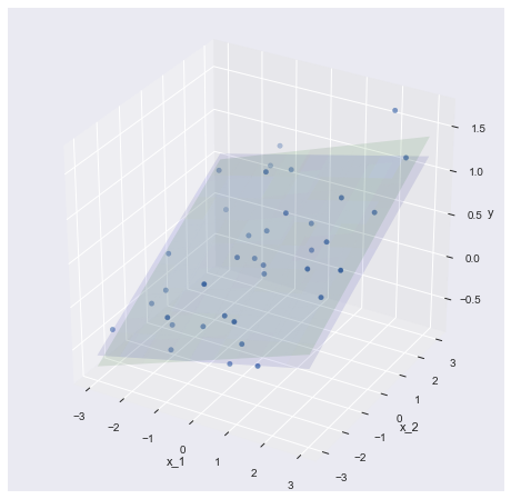
scikit-learnのLinearRegressionで重回帰する
scikit-learnのLinearRegressionを用いて
coefficientは0.15, 0.21くらい,interceptは0.35くらいとなり,
import numpy as np
from matplotlib import pyplot as plt
from sklearn.linear_model import LinearRegression
from sklearn.model_selection import train_test_split
from mpl_toolkits.mplot3d import Axes3D
from matplotlib.colors import ListedColormap

colors = ['#e74c3c', '#3498db', '#1abc9c', '#9b59b6', '#f1c40f'] # red, blue, green, purple, yellow
cmap = ListedColormap(colors)
plt.style.use('seaborn')

def f(x1,x2):
    return  0.1*x1 + 0.2*x2 + 0.3

N = 50
X = np.zeros((N,2))
np.random.seed(seed=2)
X[:,0] = np.random.uniform(-3, 3, N)
X[:,1] = np.random.uniform(-3, 3, N)
noise = 0.3*np.random.randn(N) # σ=0.3
t = f(X[:,0],X[:,1])+ noise

X_train, X_test, t_train, t_test = train_test_split(X, t, random_state=0)

fig = plt.figure(figsize=(8,8))
ax = fig.add_subplot(1,1,1, projection='3d')
ax.scatter(X_train[:,0], X_train[:,1], t_train)

lr = LinearRegression().fit(X_train, t_train)

coef = lr.coef_
line = lambda x1, x2: f(x1,x2)
grid_x1, grid_x2 = np.mgrid[-3:3:10j, -3:3:10j]
ax.plot_surface(grid_x1, grid_x2, line(grid_x1, grid_x2), alpha=0.1, color='b')

coef = lr.coef_
line = lambda x1, x2: coef[0] * x1 + coef[1] * x2 + lr.intercept_
grid_x1, grid_x2 = np.mgrid[-3:3:10j, -3:3:10j]
ax.plot_surface(grid_x1, grid_x2, line(grid_x1, grid_x2), alpha=0.1, color='g')

ax.set_xlabel("x_1")
ax.set_ylabel("x_2")
ax.set_zlabel("y")
plt.show()

print("train R^2:", lr.score(X_train,t_train))
print("test R^2:", lr.score(X_test,t_test))
print(f"coefficient:{lr.coef_} intercept:{lr.intercept_}")
単回帰と同様,二乗和誤差を小さくするような係数を探す
単回帰では1種類の
複数の教師データセット
今回はベクトルを含んだ計算が必要なので,少々トリッキーになる.
一般に,ベクトル
である.また,
これにより,
と変形できる.
と展開できる.これを
という性質があるので,
と求まる.次に,第一項目に関して考える.
一般的な
これを
「
(k,:)はnumpyのスライスと同義であり,k行の全列を抜き出した行ベクトルを表す.
これでやっと,二乗和誤差の
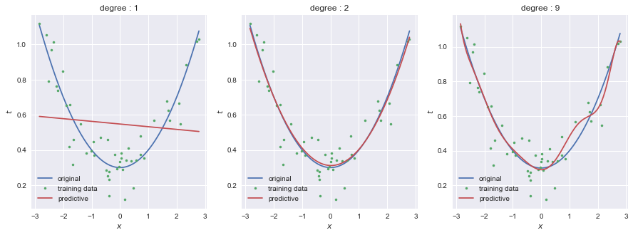
線形モデルで非線形を表現する
ここまでは,入力

結論から言うと,以下のようなモデルについて考えれば良い.
より一般化すると,
教師データを複数入力する際は,以下のような計画行列
scikit-learnのPolynomialFeaturesを用いることで,モデルの次数を自由に変えることができる.以下は1次,2次,9次の3つのモデルの結果である.
import numpy as np
from matplotlib import pyplot as plt
from sklearn.linear_model import LinearRegression
from matplotlib.colors import ListedColormap
from sklearn.pipeline import Pipeline
from sklearn.preprocessing import PolynomialFeatures
from sklearn.model_selection import train_test_split

colors = ['#e74c3c', '#3498db', '#1abc9c', '#9b59b6', '#f1c40f'] # red, blue, green, purple, yellow
cmap = ListedColormap(colors)
plt.style.use('seaborn')

def f(x):
    return  0.1*x**2 + 0.3

N = 50
X = np.zeros((N,1))
np.random.seed(seed=2)
X[:,0] = np.random.uniform(-3, 3, N)
noise = 0.1*np.random.randn(N) # σ=0.1
t = f(X[:,0])+ noise

X_train, X_test, t_train, t_test = train_test_split(X, t, random_state=0)

fig, ax = plt.subplots(1, 3, figsize = (15, 5))

for degree, ax in zip([1,2,9], ax):
    pipeline = Pipeline([
        ('polynominal_features', PolynomialFeatures(degree=degree)),
        ('linear_regression', LinearRegression())
    ])

    lr = pipeline.fit(X_train, t_train)
    print("train R^2:", lr.score(X_train, t_train))
    print("test R^2:", lr.score(X_test, t_test))
    print(pipeline.steps[1][1].coef_)

    Xcont = np.linspace(np.min(X), np.max(X), 200).reshape((200, 1))
    ax.plot(Xcont, f(Xcont), label='original')
    ax.plot(X, t,'.', label='training data')
    ax.plot(Xcont, lr.predict(Xcont), label='predictive')
    ax.set_title('degree : {}'.format(degree))
    ax.legend()
    ax.set_xlabel(r'$x$')
    ax.set_ylabel(r'$t$')
正則化項を導入することで過学習を抑える
0 < x < 1 の範囲でxをランダムに10点生成し,
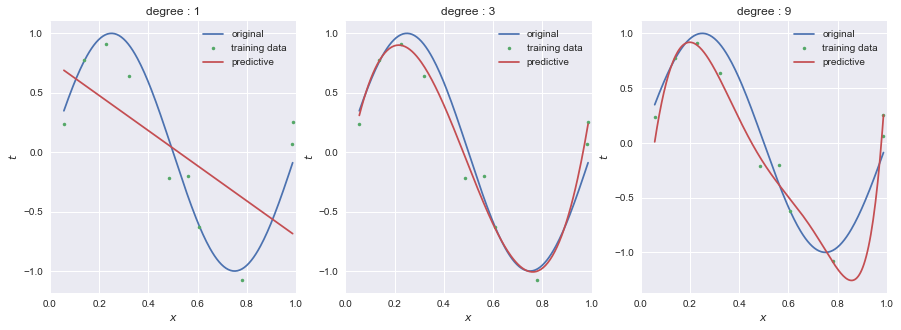
scikit-learnのLinearRegressionとPolynomialFeaturesを用いて,1次,3次,9次のモデルによって
9次において,教師データに過剰に適合しようとしていることがわかる.これが過学習(過適合,over-fitting)である.
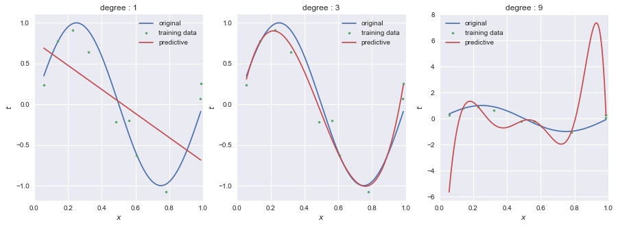
次数を小さくする(=モデルをシンプルにする)ことで過学習を避けることが期待できるが,うまい次数を探す必要がある.
教師データを増やすことで過学習を避けることができる.教師データ数を10組から100組に増やした例が以下であり,9次のモデルでも予測できている.
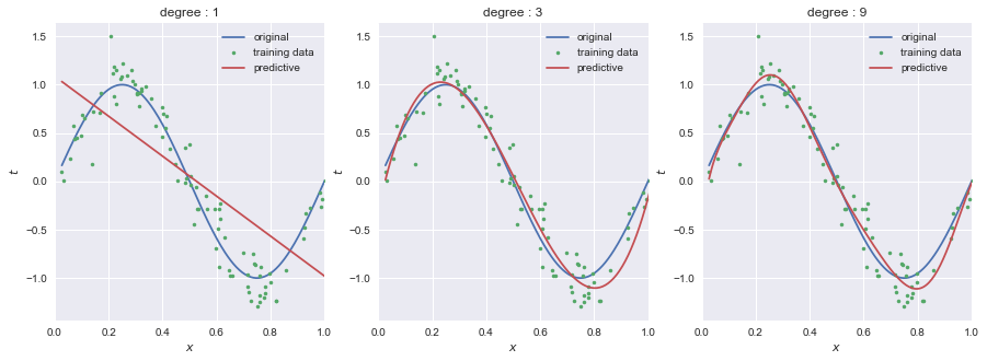
教師データが大量に手に入る場合はいいかもしれないが,限られた量しか手に入らない場合は断念しなければならないといった問題がある.
ここで,各次数のモデルにおける係数
| | | | | | | | | |
|---|---|---|---|---|---|---|---|---|---|
| 0.0 | -2.1 | ||||||||
| 0.0 | 12.6 | -35.3 | 22.7 | ||||||
| 0.0 | 22.2 | -263.1 | 2140.3 | -9774.9 | 25228.6 | -38193.9 | 33691.2 | -16021.9 | 3171.9 |
過学習である/ないに関わらず,モデルの次数が大きくなるほど係数wが大きくなっている.つまり,小さいノイズが誇張されてしまうので,過学習が発生すると考えることができる.
より論理的には,
そこで,単位行列
これは,以下の二乗和誤差を最小にする値である.
scikit-learnのRidgeを用いてRidge回帰を行った結果が以下である.過学習が抑えられている.
Ridgeには,
9次のモデルにおいて,
import numpy as np
from matplotlib import pyplot as plt
from matplotlib.colors import ListedColormap
from sklearn.pipeline import Pipeline
from sklearn.preprocessing import PolynomialFeatures
from sklearn.linear_model import Ridge

colors = ['#e74c3c', '#3498db', '#1abc9c', '#9b59b6', '#f1c40f'] # red, blue, green, purple, yellow
cmap = ListedColormap(colors)
plt.style.use('seaborn')

def f(x):
    return  np.sin(2*np.pi*x)

N = 10
X = np.zeros((N,1))
np.random.seed(seed=3)
X[:,0] = np.random.uniform(0, 1.1, N)
noise = 0.2*np.random.randn(N) # σ=0.2
t = f(X[:,0])+ noise

X_train, X_test, t_train, t_test = train_test_split(X, t, random_state=0)

fig, ax = plt.subplots(1, 3, figsize = (15, 5))

for degree, ax in zip([1,3,9], ax):
    pipeline = Pipeline([
        ('polynominal_features', PolynomialFeatures(degree=degree)),
        ('ridge', Ridge(alpha=0.0000001))
    ])

    lr = pipeline.fit(X_train, t_train)
    print("train R^2:", lr.score(X_train, t_train))
    print("test R^2:", lr.score(X_test, t_test))
    print(pipeline.steps[1][1].coef_)

    Xcont = np.linspace(np.min(X), np.max(X), 200).reshape((200, 1))
    ax.plot(Xcont, f(Xcont), label='original')
    ax.plot(X, t,'.', label='training data')
    ax.plot(Xcont, lr.predict(Xcont), label='predictive')
    ax.set_xlim(0.0, 1.0)
    ax.set_title('degree : {}'.format(degree))
    ax.legend()
    ax.set_xlabel(r'$x$')
    ax.set_ylabel(r'$t$')